on
Week 5: The Air War
Intro
For this week’s blog post, I looked at the role of advertisements in predicting election outcomes. Media can serve to persuade and convince voters to turnout through a variety of methods. This can create an “air war” as each party attempts to have their media prevail. What is the scale of this “war”? Well, in 2018, it is estimated that in total $529,716,980 were spent on ads (WMP: ads_issues_2012-2018.csv). This leads to the question of what differences arise between the Democrat and Republican parties’ use of media? What does the “air war” look like at a district level? Finally, how strong of a predictor is money spent on advertisements on election outcomes?
Data
To answer these questions, I primarily looked at data from the Wesleyan Media Project. The data set included all political ads ran between 2012 and 2018. The variables I used in this data set include the state, district, and year of each ad. I also looked at the estimated cost and the party associated with each ad. To build off the data from past weeks, I included average expert rankings and actual vote share for each district. With this data, I first look at the money spent on ads in each district broken down by party. I then predicted the democratic vote share outcome in each district by modeling the average cost spent on ads and the expert rankings (continuing last week’s data). Finally, I provide an update on my prediction for nationwide party vote share.
## Rows: 16067 Columns: 31## ── Column specification ────────────────────────────────────────────────────────
## Delimiter: ","
## chr (16): Office, State, Area, RepCandidate, RepStatus, DemCandidate, DemSta...
## dbl (14): raceYear, RepVotes, DemVotes, ThirdVotes, OtherVotes, PluralityVot...
## lgl (1): CensusPop##
## ℹ Use `spec()` to retrieve the full column specification for this data.
## ℹ Specify the column types or set `show_col_types = FALSE` to quiet this message.## Rows: 148 Columns: 6## ── Column specification ────────────────────────────────────────────────────────
## Delimiter: ","
## chr (1): state
## dbl (5): district, ave_cost, ave_ads, total_dem, total_rep##
## ℹ Use `spec()` to retrieve the full column specification for this data.
## ℹ Specify the column types or set `show_col_types = FALSE` to quiet this message.Money Spent on Ads
Democrats
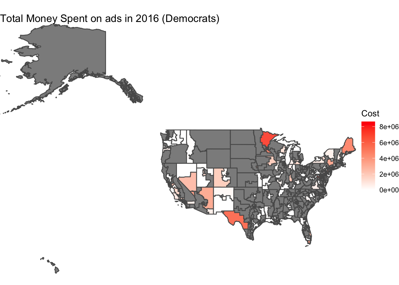
In the map below, I show the total estimated cost of advertisements Democrats spent in each district during the 2016 election.
Republicans
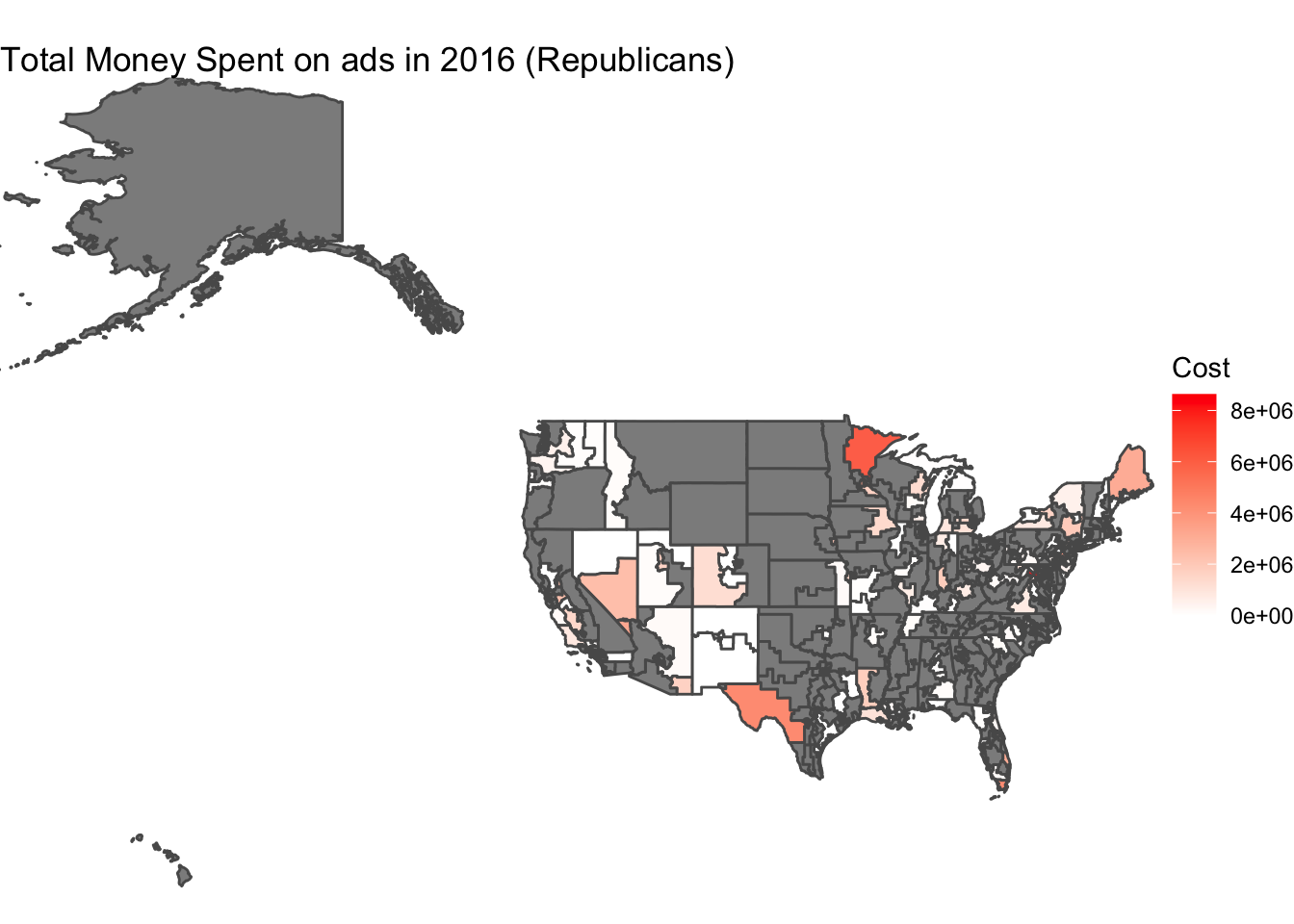
In the map below, I show the total estimated cost of advertisements Republicans spent in each district during the 2016 election.
 ## Comparison
These maps show that, generally, the parties focus on the same districts with their advertisements. The districts with the greatest difference between party ads include Arizona 1, New York 19, and Texas 23. For these districts, the Democratic party spent more than the Republican. Additionally, from this map we see that the most money on ads was spent in Minnesota 8. Although these maps give a general idea of the trends for how each party spends ad money, a better way to do this would have been to map the number of ads in each district. This is because the costs are only estimates and do not provide a great display of the effect of the prevalence of ads in the district.
District Level Modeling
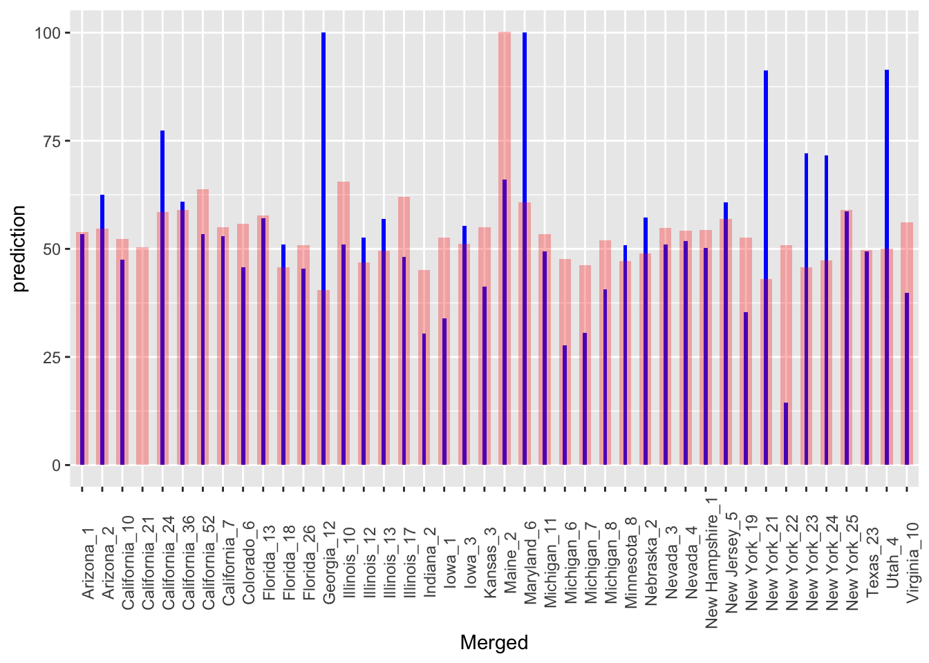
To see how well of a predictor ad cost is for democratic vote share, I ran a regression model for each district. Due to the lack of data from 2022, I looked at all years except 2018 and used 2018 as the predictor data. The results can be seen in the plot below. The red column represents the predicted democratic vote share and the blue line represents the actual vote share.
##
## Call:
## lm(formula = DemVotesMajorPercent ~ prediction, data = pred_2022_plot)
##
## Residuals:
##     Min      1Q  Median      3Q     Max
## -11.994  -3.209  -0.254   2.911  13.085
##
## Coefficients:
##              Estimate Std. Error t value Pr(>|t|)
## (Intercept) 5.249e+01  2.378e+00  22.076   <2e-16 ***
## prediction  1.913e-04  4.269e-02   0.004    0.996
## ---
## Signif. codes:  0 '***' 0.001 '**' 0.01 '*' 0.05 '.' 0.1 ' ' 1
##
## Residual standard error: 5.57 on 41 degrees of freedom
## Multiple R-squared:  4.899e-07,  Adjusted R-squared:  -0.02439
## F-statistic: 2.009e-05 on 1 and 41 DF,  p-value: 0.9964
Analysis
Visually, it is apparent that there is a lot of variation between the predicted and actual value. This is confirmed by the extremely low R squared value of approximately 0. Additionally, there are some predicted values that are over 100% and less than 0%. This is very indicative of a faulty model and can possibly be attributed to the inconsistency in spending patterns over the years. Further, the prediction model does not consider if there is no challenger. This is a problem because for those districts, the vote share will be near the extremes. However, my model predicts most of the districts to be around 50%.
When I add in expert ratings from last week, the regression shows a slight positive correlation between money spent and democratic vote share. However, the R squared value is 1, making this model have no significance.
Overall, the usage of ad costs proves not to perform well as a predictive variable. This observation has some similarities with the results in the piece, “How Large and Long-lasting Are the Persuasive Effects of Televised Campaign Ads?” In this article they claim that the long-term effects of advertisements are not that strong (Gerber et al., 2011). This could be indicative of why there is such a weak correlation shown in my model.
Updated Natiowide Model
Instead of incorporating ads into my model, I chose to revert back to my model for nationwide vote share from week 3. I updated the polls from 538’s generic poll. The model predicts republicans having 48.31384 of the vote share and democrats having 48.4402. This is a much smaller margin than last week, but still has democrats winning over republicans.
## New names:
## * `` -> ...1
## Rows: 435 Columns: 9## ── Column specification ────────────────────────────────────────────────────────
## Delimiter: ","
## chr (4): District, cpr, inside_elections, crystal_ball
## dbl (5): ...1, cpr_num, inside_elections_num, crystal_ball_num, avg##
## ℹ Use `spec()` to retrieve the full column specification for this data.
## ℹ Specify the column types or set `show_col_types = FALSE` to quiet this message.## New names:
## * `` -> ...1
## * ...1 -> ...2## Rows: 3284 Columns: 23## ── Column specification ────────────────────────────────────────────────────────
## Delimiter: ","
## chr (2): party, winner_party
## dbl (21): ...1, ...2, year, quarter_cycle, GDP_growth_qt, DSPIC_change_pct, ...##
## ℹ Use `spec()` to retrieve the full column specification for this data.
## ℹ Specify the column types or set `show_col_types = FALSE` to quiet this message.##
## Call:
## lm(formula = R_totalvote_pct ~ CPIAUCSL.ave + R_support, data = fundamentals_polls.Oct)
##
## Residuals:
## Min 1Q Median 3Q Max
## -7.6599 -1.8073 0.3795 1.6727 6.2816
##
## Coefficients:
## Estimate Std. Error t value Pr(>|t|)
## (Intercept) 37.455697 0.493470 75.903 <2e-16 ***
## CPIAUCSL.ave -0.001802 0.001210 -1.489 0.137
## R_support 0.255971 0.012195 20.989 <2e-16 ***
## ---
## Signif. codes: 0 '***' 0.001 '**' 0.01 '*' 0.05 '.' 0.1 ' ' 1
##
## Residual standard error: 2.396 on 1641 degrees of freedom
## (1640 observations deleted due to missingness)
## Multiple R-squared: 0.2213, Adjusted R-squared: 0.2204
## F-statistic: 233.2 on 2 and 1641 DF, p-value: < 2.2e-16##
## Call:
## lm(formula = D_totalvote_pct ~ CPIAUCSL.ave + D_support, data = fundamentals_polls.Oct)
##
## Residuals:
## Min 1Q Median 3Q Max
## -5.6424 -2.1728 -0.4015 2.0968 7.7139
##
## Coefficients:
## Estimate Std. Error t value Pr(>|t|)
## (Intercept) 39.865075 0.688039 57.940 < 2e-16 ***
## CPIAUCSL.ave -0.008382 0.001362 -6.156 9.37e-10 ***
## D_support 0.243458 0.013052 18.652 < 2e-16 ***
## ---
## Signif. codes: 0 '***' 0.001 '**' 0.01 '*' 0.05 '.' 0.1 ' ' 1
##
## Residual standard error: 2.806 on 1637 degrees of freedom
## (1644 observations deleted due to missingness)
## Multiple R-squared: 0.2062, Adjusted R-squared: 0.2052
## F-statistic: 212.6 on 2 and 1637 DF, p-value: < 2.2e-16## 1
## 48.31384## 1
## 48.4402