on
Week 6: The Ground Game
Intro
For this week’s blog post, I looked at how campaigns can contribute to the outcome of the election. These efforts, characterized as the “ground game” seek to coordinate volunteers through local field offices in hopes of persuading people and supporters to vote Darr and Levendusky, 2014. With the vast number of people and resources that go into campaigning, it begs the question of how important is turnout in elections? Can turnout be used to predict elections at a district level? This week I also look at updating my district level model. The main question I consider is how to include districts that have limited data in my model?
Data
The data I used this week involves a lot of data introduced in previous blog posts. The main new dataset that I use this week is CVAP data. This provides the Citizen Voting Age Population for each data. I use this variable, along with the actual vote numbers during the elections, to get the turnout rate for each district. For districts without CVAP data, I use nationwide turnout rates. With regard to updating my model, I continue to use CPI rates (Week 2), generic ballot polls (Week 3), and expert ratings (Week 4). Finally, I work with the actual House election results by district from 1948 to 2020.
## Warning in sprintf("https://cdmaps.polisci.ucla.edu/shp/districts114.zip", :
## one argument not used by format 'https://cdmaps.polisci.ucla.edu/shp/
## districts114.zip'
## Warning in sprintf("districtShapes/districts114.shp", cong): one argument not
## used by format 'districtShapes/districts114.shp'## Reading layer `districts114' from data source
## `/private/var/folders/ds/13_jz5hd0y719qz96prb8mzm0000gn/T/RtmpOiODWq/districtShapes/districts114.shp'
## using driver `ESRI Shapefile'
## Simple feature collection with 436 features and 15 fields (with 1 geometry empty)
## Geometry type: MULTIPOLYGON
## Dimension: XY
## Bounding box: xmin: -179.1473 ymin: 18.91383 xmax: 179.7785 ymax: 71.35256
## Geodetic CRS: NAD83Turnout
Turnout Only Model
I first looked at turnout as the single predictor variable for each district. In order to produce 435 predictions, I had to ensure each district had a turnout value. For the majority of districts that fell within the CVAP data set, I divided the total votes for each election and divided by the cvap value. For the districts without a cvap value, I used the national turnout value. For the predicted value, I used the 2018 data because it is the last midterm election.
The map below shows the predicted seat distribution. Democrats win 222 seats.
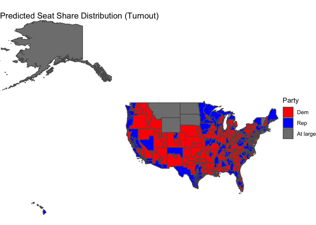
Democrats gaining the majority of seats in this model correlates to conclusions that I drew last week. Last week, I looked at the “air war” and different spending patterns the parties had toward advertisements. I noticed that Democrats appeared to spend more money than Republicans in competitive districts. This idea relates to Enos and Fowler’s piece “Aggregate Effects of Large-Scale Campaigns on Voter Turnout,” in which they argue that campaigning can increase turnout by 7-8 percentage points. Therefore, if advertisement spending is somewhat reflective of overall campaign expenditures in a district, then it makes sense that Democrats would invest in campaigning that results in a higher turnout and delivers a majority in the House (as seen by the prediction model). Ultimately, higher turnout appears to give democrats an advantage.
However, the average adjusted R-squared among these regressions was 0.021, so extremely low. This means that turnout alone is not a good enough predictor.
Turnout and Other Variables:
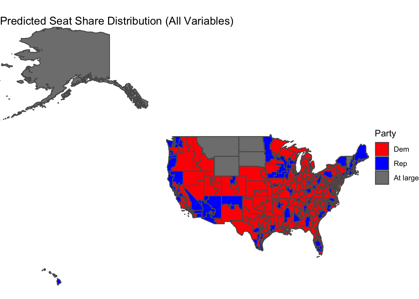
I then reintroduced my previous variables to the model. This includes average polling, incumbency, and expert ratings. To ensure each district could be modeled, I had to handle NAs. The following shows my thought process: –NAs for polling: use nationwide generic ballot for that year –NAs for incumbency: code as a -1 –NAs for expert ratings: use 2018 data which is exhaustive for each district
This map shows Democrats winning 214 seats. The average adjusted R-squared is 0.2346256, which is significantly higher than the turnout only model, however still fairly low.
Differnce
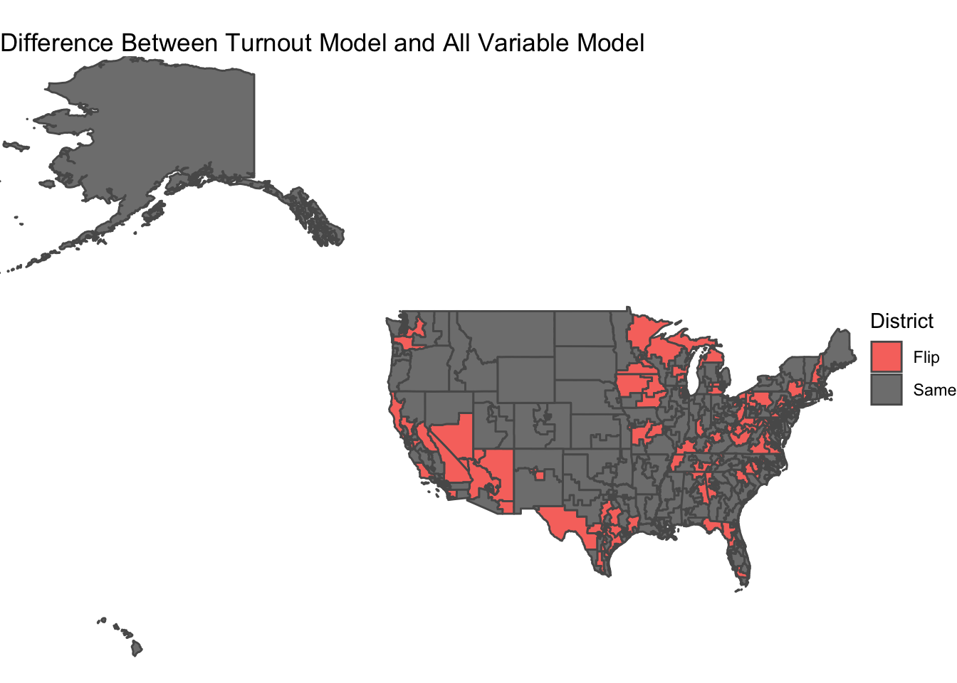
The map below shows the difference between the two models (Turnout only and the all variable model). There were a total of 115 flipped districts, but only a net decrease of 7 seats for democrats.
Updated Prediction
For this week, I will be using the results from the previous model to update my prediction. The model predicts Democrats winning 214 seats and Republicans with 221 seats.
Conclusion and Limitations
This week I looked at adding turnout to my model. Turnout alone was a poor predictor. This can be attributed to numerous factors. Some of the most prominent include that for many districts, I used the national turnout rate which was probably much higher than most of the small, rural districts where data is limited. Further, with limited years, the data had lots of fluctuation and overall inconsistencies that could contribute to its lack of predictive power.
This is the first week that my model has predicted Republicans winning. This appears to be more in line with what other major polls are showing, such as [FiveThirtyEight])(https://projects.fivethirtyeight.com/2022-election-forecast/house/) and The Economist.
Moving Forward
In the future, I will continue to update my district level model. With a low adjusted R-squared, I will be looking to make my variables more predictive. One area that I think will help will be to continue considering how to deal with NAs.