on
Week 7: Shocks
Intro
As the Midterms get closer, I have to start being more critical of my model and put the finishing touches on it. This is my last blog post before I share my final prediction and model. For this reason, this week I mainly look at improving my model, by adjusting my variables. I decided to revert back to my national vote share prediction from earlier blogs after last week. Although I was able to model each district, due to the lack of robust data in the majority of districts, I ended up using a lot of nationwide data to fill in the holes. For example, where polling was limited, I used the generic ballot. This made the adjusted R-squared value to be very small or equal to 1 because districts were often being modeled off of one or two previous elections. Aside from improving my model, I also look at shocks in this election cycle. I do not intend to include this in my model because shocks are inherently not predictive, however, it is interesting to see what, if any, impacts shocks have on polling averages.
Data
The main variables I add in my model this week are demographics. I used data from the US Census to see how well race, gender, and education background can serve as variables in the model. This data is from 1964 to 2020 and includes the demographics of past voters. Additionally, I continue to use data on DSPIC (Disposable income), CPI, and polls. For looking at shocks, I used the New Times database to see the number of articles published on a certain topic.
Shocks
In lecture and lab this week we studied the impact of the Dobbs v. Jackson Women’s Health Organization decision, which effectively overturned Roe v. Wade, placing the states in power to determine one’s right to abortion. This decision was initially leaked in early May and then officially released about a month later. In lab, we saw an initial spike in number of articles when the draft was leaked and then a much larger spike when the actual draft was released. However, this trend was not as evident in the polling averages during this time. There was a slight peak in democratic vote share after each release, but that tended to fade back to the normal trend within a week. Over shocks that could be considered during this time are nationwide ones such as the Raid of Mar-a-lago. However, it is also important to consider that local shocks may be even more significant to voters. For example, the health of Candidate John Fetterman could impact Pennsylvania voters or the scandals about Herschel Walker may be important to Georgia voters. Shocks do matter in elections (Achen and Bartel (2017)), however, it is difficult to really what constitutes as a shock before the election.
Model Updates: How I improved my model
Fundamentals
The first thing I did to improve my model was look at the logarithmic relationship between a variable and Democratic vote share. For the economic fundamentals, I found that when I took the log of DSPIC, the R-squared increased by 0.3%. This made DSPIC the strongest predictor among GDP, CPI, and Unemployment. I kept the filtering to be for the 7th economic quarter of the election cycle
Demographics
I then looked at included demographic data into my model. I first looked at the percentage of Black and White voters. When I included these variables I found that the R-squared went significantly higher (0.7), but none of the coefficients were significant. I then looked at gender.
Gender
I found that including the log value of percent female and log value of percent male, while holding the log value of percent male constant to prevent collinearity, improved my model’s R-squared value and coefficients. R-squared = 0.56.
Education
Using a similar approach as I did with gender, I then included the log of college educated voters and log of no GED voters. I similarly held no GED constant to prevent collinearity. The R-squared increased to 0.65.
Years
I then wanted to see how my model changed if I subsetted the years to just midterm years. I found that the R-squared increased to 0.73.
##
## Call:
## lm(formula = D_seats ~ D_support + DSPIC_change_pct + log(`Femal CVAP`):log(`Male CVAP`) +
##     log(College):log(`No GED`), data = dataDMid)
##
## Residuals:
##     Min      1Q  Median      3Q     Max
## -17.570 -11.792  -1.214  15.931  19.780
##
## Coefficients:
##                                    Estimate Std. Error t value Pr(>|t|)
## (Intercept)                         540.555    476.041   1.136   0.2935
## D_support                             4.688      1.892   2.477   0.0424 *
## DSPIC_change_pct                      5.027     12.331   0.408   0.6957
## log(`Femal CVAP`):log(`Male CVAP`)  -59.458     41.925  -1.418   0.1991
## log(College):log(`No GED`)           30.109     16.596   1.814   0.1125
## ---
## Signif. codes:  0 '***' 0.001 '**' 0.01 '*' 0.05 '.' 0.1 ' ' 1
##
## Residual standard error: 17.63 on 7 degrees of freedom
##   (3 observations deleted due to missingness)
## Multiple R-squared:  0.833,  Adjusted R-squared:  0.7376
## F-statistic:  8.73 on 4 and 7 DF,  p-value: 0.007451
##
## Regression Results
## ================================================================
## Dependent variable:
## -----------------------------------
## Democratic Major Vote Share Percent
## ----------------------------------------------------------------
## Polls 4.7**
## (1.9)
##
## Disposible Percent Income Q7 5.0
## (12.3)
##
## Female Percent -59.5
## (41.9)
##
## Male Percent 30.1
## (16.6)
##
## College 540.6
## (476.0)
##
## ----------------------------------------------------------------
## Observations 12
## R2 0.8
## Adjusted R2 0.7
## Residual Std. Error 17.6 (df = 7)
## F Statistic 8.7*** (df = 4; 7)
## ================================================================
## Note: *p<0.1; **p<0.05; ***p<0.01Analysis:
The above output has a fairly significant adjusted R squared value and p-value. However, the extremely high intercept indicates the output is not very significant. Although, looking at the coefficients, it is evident that the Fermale:Male and College:No GED interaction terms have the strongest predictive power. Moving forward, these will be important demographics to consider in my model.
Prediction:
To predict national vote share, I used demographics from 2020, which is the most recent census, DSPIC from today (0.1), today’s polling from 538 (44.8).
My model predicts democrats with 52.13964 percent of the vote share.
Prediction Intervals
My prediction intervals are: 47.12753 - 57.15176
This is a fairly large prediction interval, especially with regard to elections when vote share can come down to a difference of a fraction of percent. I think the limited years of data definitely contributes to this problem. However, decreasing this interval will be important.
##        fit      lwr      upr
## 1 240.6438 186.5373 294.7503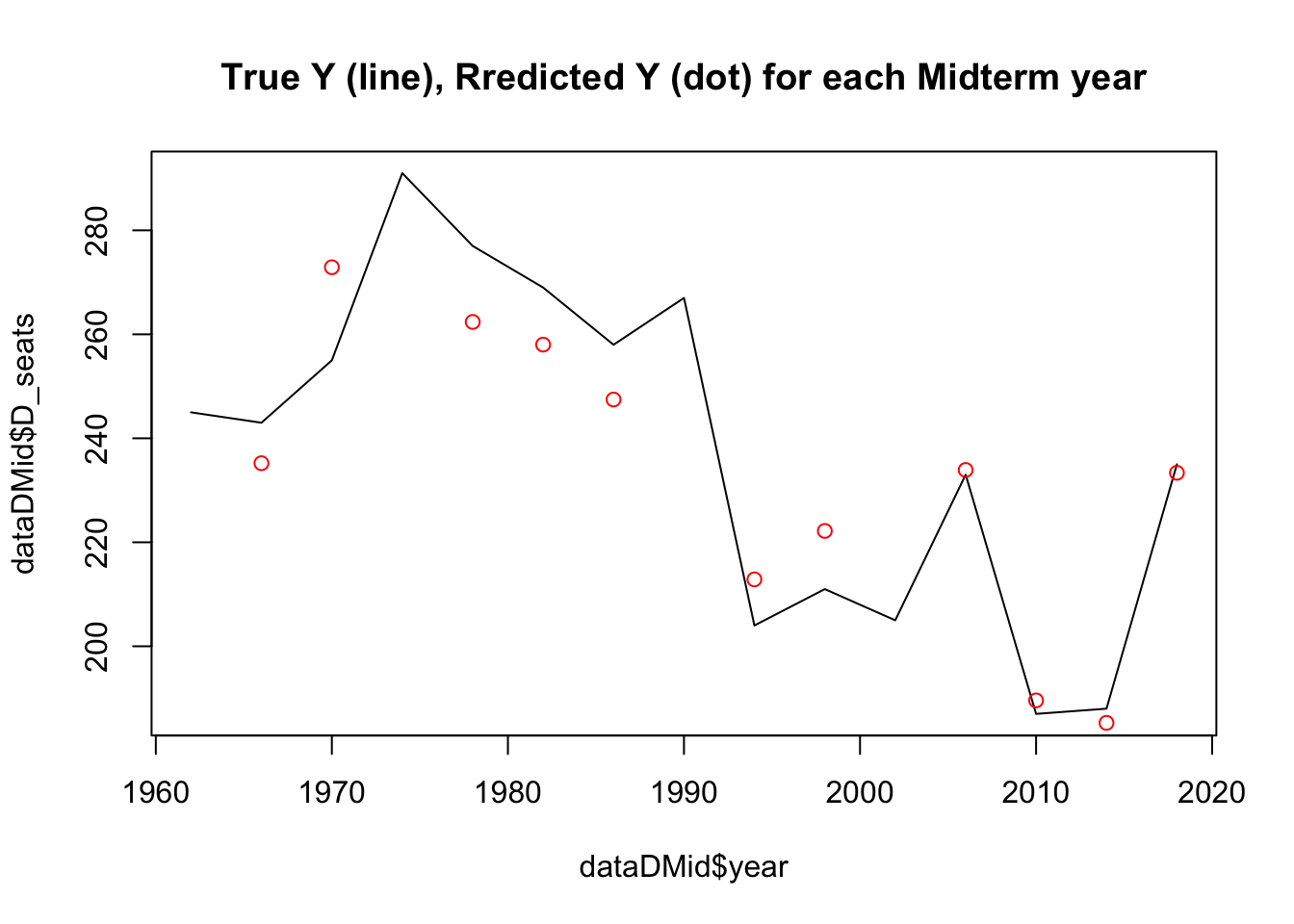
Limitations
The main limitation in my model is lack of data. When I filtered for midterm years, my model improved, however, it is only using data from 16 past elections. This is not nearly enough for me to be confident it will accurately assess new data. Further, the demographics in my model are from 2020. This is not that accurate because the electorate who votes in presidential elections versus midterms can differ by a lot. I chose to use 2020 versus 2018 because I felt that having the most recent demographic data was important, however, I recognize the trade-off that these demographics can differ.
Moving Forward:
Between now and election day, I will continue to improve my model. I also am going to look at a few districts that have a lot of data and build individual models for them. This will not be my main prediction, but it will allow me to see if my nationwide model has any predictive power at the district level.